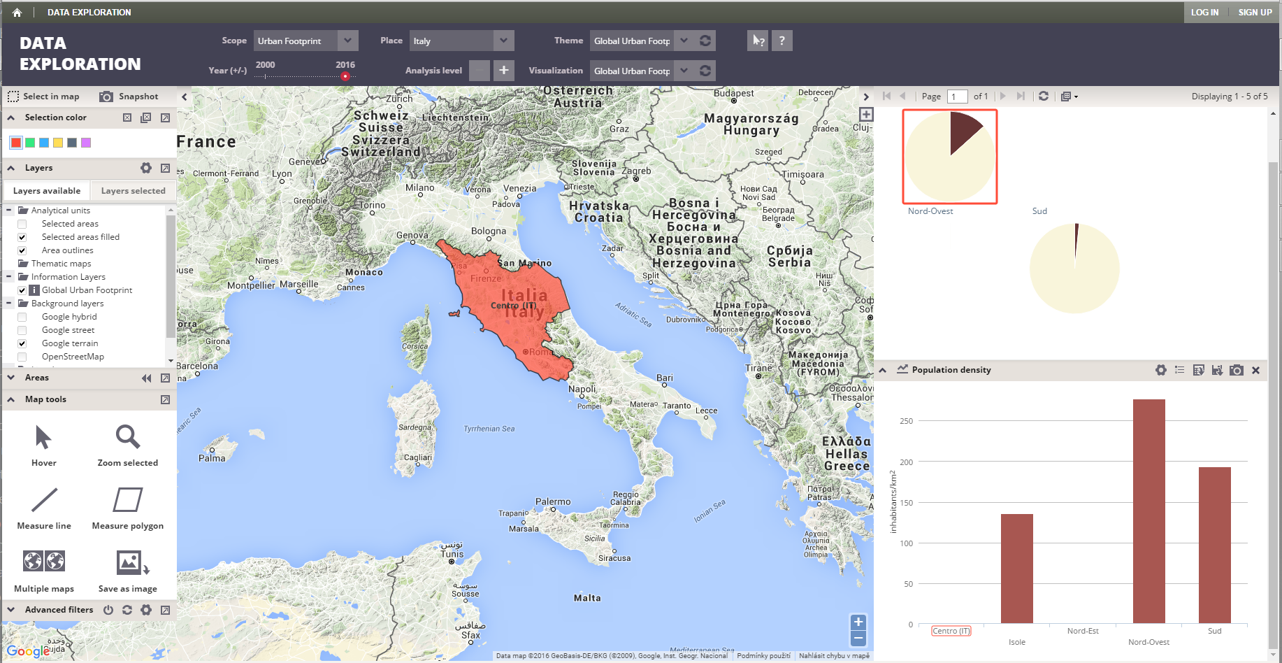
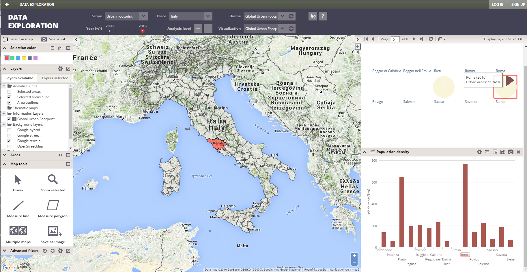
PUMA Exploration interface allows examination of various spatial data. Multiple map layers can be displayed, both static from local or remote sources and dynamically created choropleths from corresponding attributes. Aside from the map, attribute data can be also displayed in multiple graphs and/or tables, including optional normalizations.
The layers and their attributes are organized in the Scopes. Scopes explain the size of the areas ready for the analysis. An example of such Scope is Global, which contains global products organized into the Places. The places represent an analytical units combined with the area they belong to. In Global Scope it is meaningful to organize the places alongside the country boundaries for example. The Scope is also organized around the concept of Themes. Theme represent certain subset of visualisations to show to the user. Visualisation is combination of the shown layers, the area which is shown on the map and the charts alongside.
In the example in the image we chose Local Scope meaning that the data are focused on local areas such as cities. As a Place we selected Cebu City, thematically we are interested in data related to Land Cover and the charts and the layers shown belong to the visualisation of the structures.

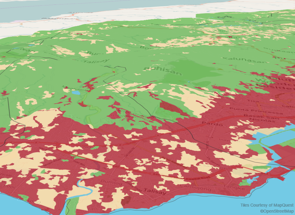
The map is available as a 2D as well as 3D. Tha main purpose of the map is to display the data sets as image data on top of the map. The data sets are organized as explained in Top panel - data selection. They are also further structured in the layer groups in the panel.
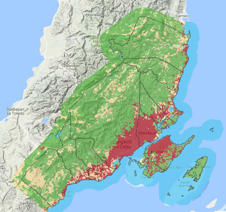
On the map, the tool can display various background layers (e.g. OpenStreetMap, Google Earth), raster and vector layers both uploaded into the tool or from remote sources (if exposed as WMS), and area layers - boundaries and selections.
In this part we explain the tools available under the top panel. All these tools can be shown floating or hidden in the panel.
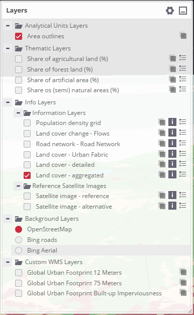
In the tool it is possible to see the available layers and select the ones to be visible in the map. For each layer it is possible to show the metadata information associated with the layer, show and hide a legend and specify the opacity of the layer.
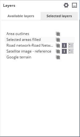
For selected layers it is possible to order them using tool depicted on the next image. The ordering happens by using drag and drop.
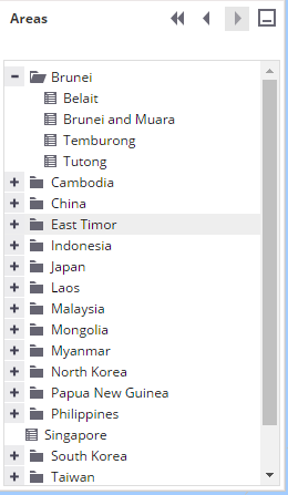
The analytical units are grouped into the levels. This tool allows you to see the units associated with given area structured as a tree based on the levels.
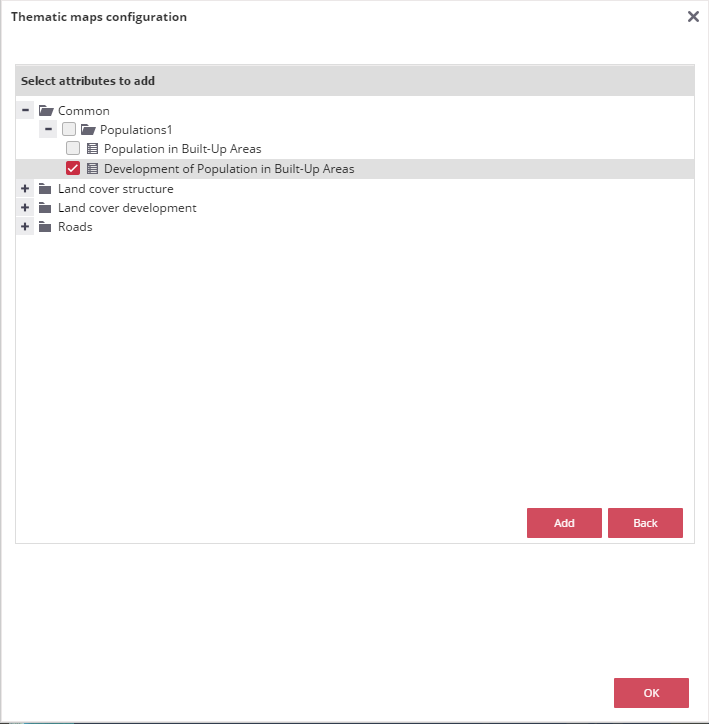
The layers contain attributes, which can be used as the source of the data for the charts displayed in the right part. There are 4 types of charts supported. Each chart can show one or more attributes. The exact display differs based on the type of the chart. It is also possible to specify the units which will be displayed in the chart and adapt them by using custom factor to multiply the values.
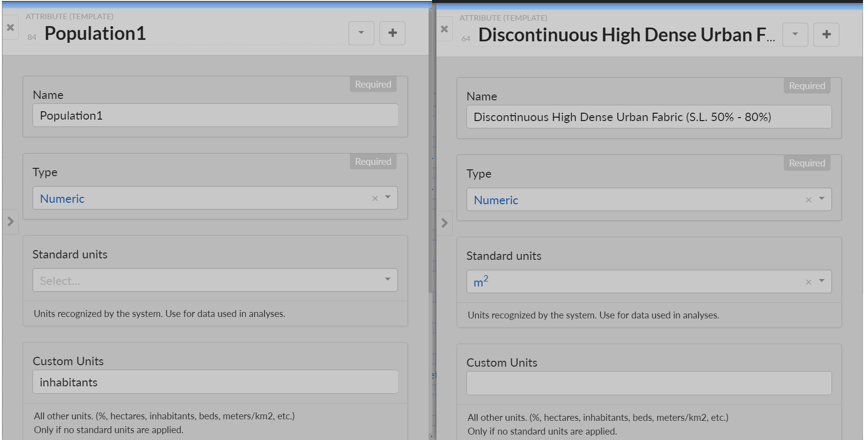
There are two places which are important with respect to units in BackOffice. First is setting the units of the attribute. These units represent in which units the attribute is represented in the data. These units are also shown without any normalization or update to units in the FrontOffice charts.
When creating or updating the attribute it is possible to specify the units. There are two types of units. Standard units and custom units. It is always possible to set only either standard units or custom units. These units express what units the values in the data are. They are also by default shown in the charts.
It is important to take into account units for the spatial aggregation analysis. Depending on the exact type of the analysis there are multiple units, which can be taken into account.
No changes
In this case it either counts the amount of units in all more detailed units or sums all attributes in the given area. There is no change in the units and in the FrontOffice they are shown as explained in further section.

Normalization over area
Handling of this dependts on whether the units of target attribute are standard or custom. If the units are standard, then the result which is counted in m2 is transformed to the target unit by dividing it using appropriate number. If the units are nonstandard the data remains unchanged after the operation itself.

Attribute weighted by area
In this case there is one attribute, which is relevant for the operation and the resulting attribute. If both of these attributes are in standard units, it is possible to update resulting value by the fraction representing the relationship between all three units. One of them is source units, second is area which is always in m2 and third is resulting attribute. Basically the whole process goes as:
If any of the attributes is non standard no operation happen on the result.

Attribute weighted by another attribute
This use case is very similar to the previous one, except that instead of the m2 unit of the area there is unit of the third attribute.

The source unit for an attribute is set in the BackOffice. This source unit says what unit is the representation of the data in.
In the FrontOffice, it is possible to display the values stored under the attributes using different type of charts. There are multiple ways how the values could be adapted before the final display of the chart to the user. The simplest way is to simply show the values using table.
Show the values without changes
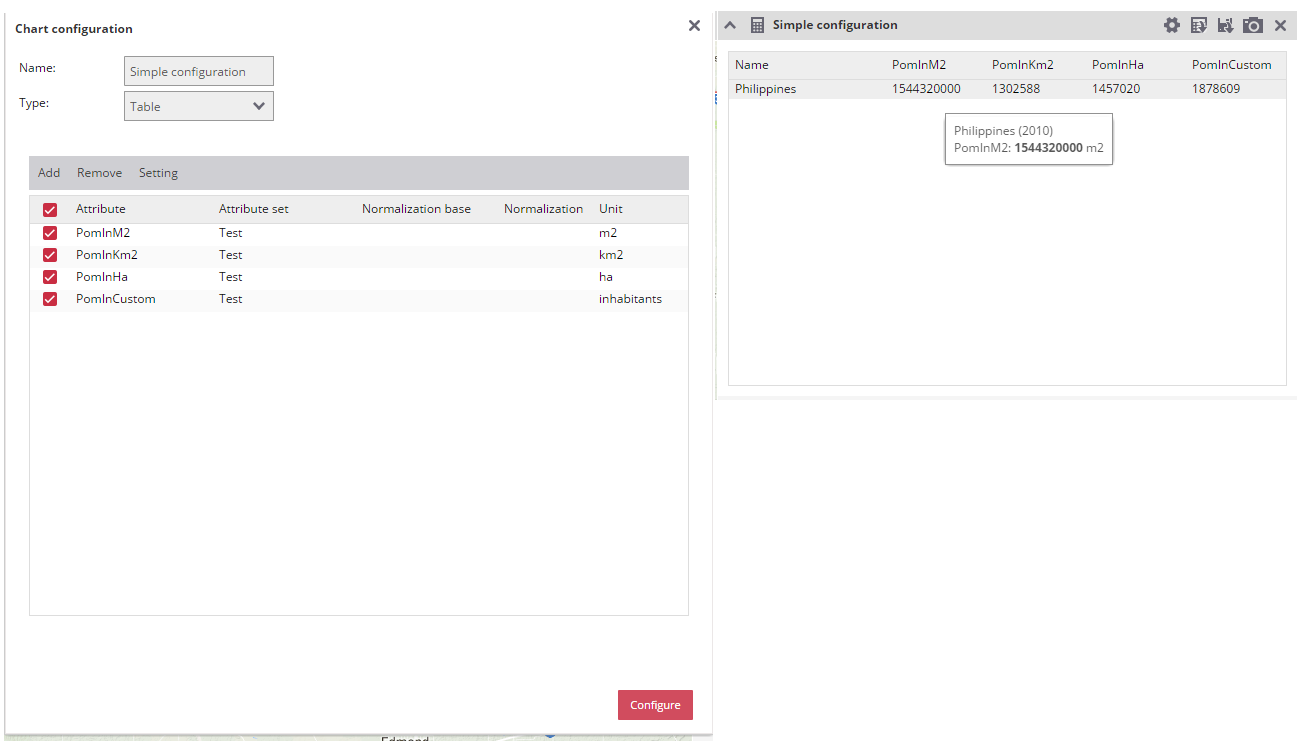
For this use case it is enough to open the configuration of the chart. Choose the correct type of the chart and select the attributes, which will be visualised. The units which will be shown in the legend are the same as in the BackOffice. For the reference they are also displayed in the table of atributes to display in the chart.
Table
Column
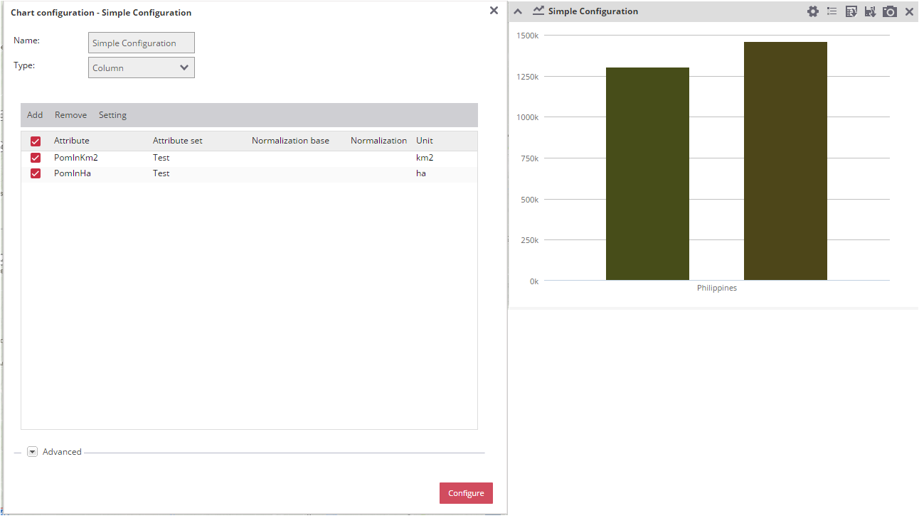
Show the values changed to different display unit.
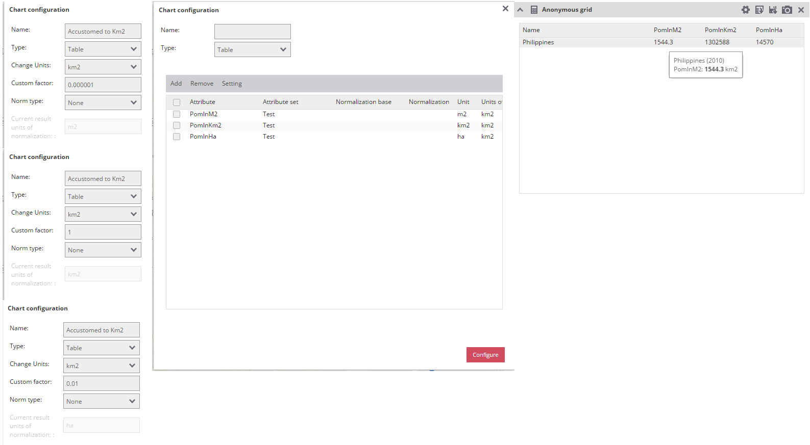
This use case allows you to display the data in different units than the source one provided to the attribute in the BackOffice. First example will show how to update all shown attributes so that they are displayed in the km2 instead of the default units.
There two important things that these settings does. The first one is changing the unit in the legend. This is done via the select Change Units. If you select some unit here, this is the unit which will be displayed in the legend. The second one is to update the values to a different one before showing the value to the user. This is handled via the Custom Factor field. This scenario has two options. First is that the source units are recognized by the system in which case the custom factor will be filled by the default factor. If the source units aren’t recognized by the system the factor will be filled by 1 by default. It is possible to use any factor as long as it is number. The value is simply multiplied by the factor before being returned for display.
Table
Show the values normalized to the area
In this use case you have attribute in any units and want to show the statistical information based upon the area. This have again two possible ways to be displayed. First is that the units of the source attribute is standard supported by the system. Second is that the units of the source attribute are in nonstandard units such as inhabitants.
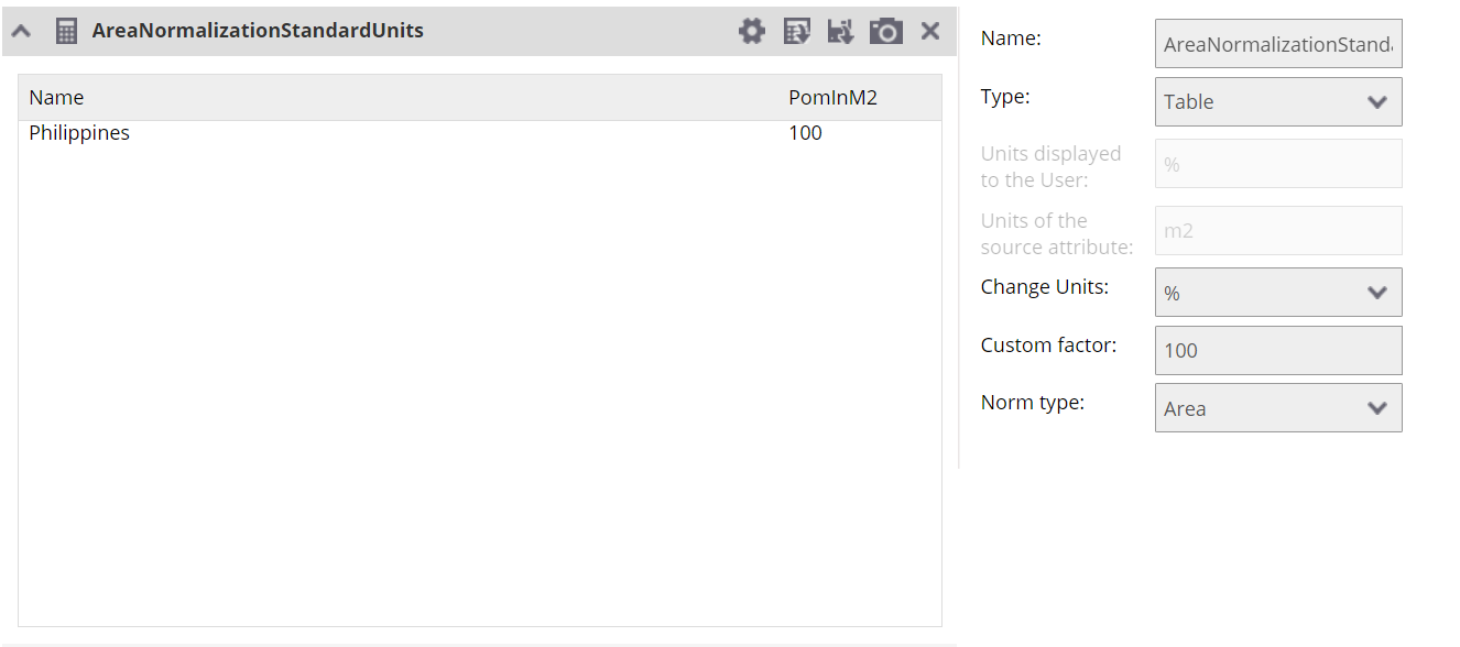
Source units are standards
In this case the default resulting unit is %. Unless you change the unit to one of the standard and/or update the custom factor, the value in the data will be divided by the area, adapted to difference in units and then multiplied by 100 and % is shown as the unit.
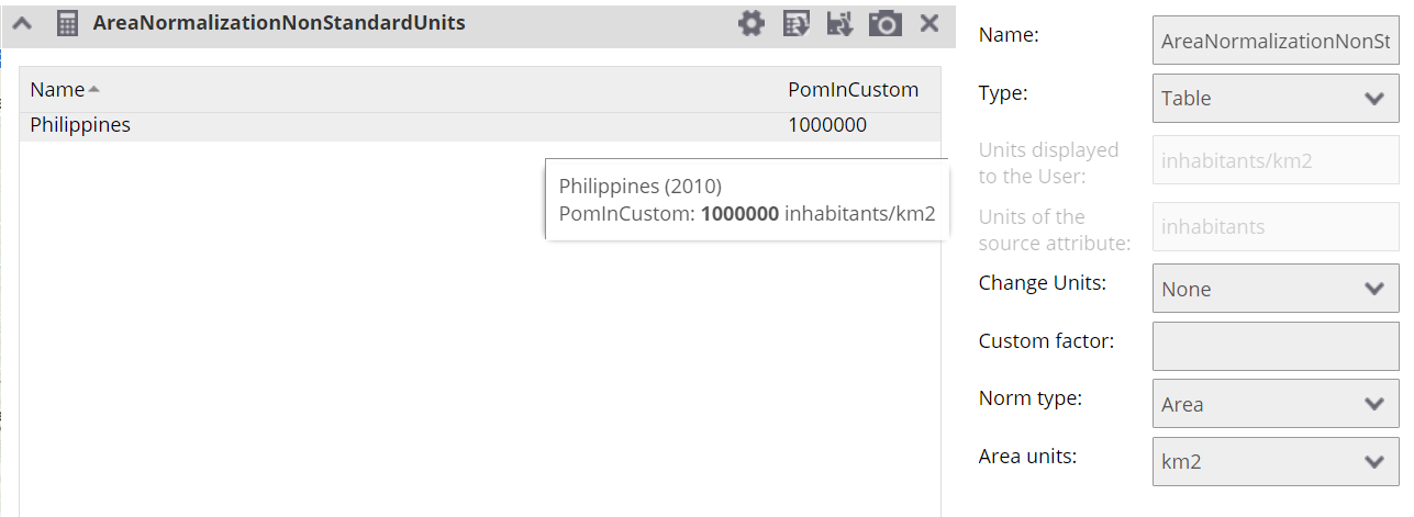
Source units are nonstandard
In this case there is one more setting to take into account. It is possible to select the units over which the default values will be normalized. If for example we have the source attribute in inhabitants as units, the default resulting unit will be inhabitants/m2. It is possible to specify other standard units changing the result for example to inhabitants/km2.
Show the values normalized to the attribute set
The normalization is happening against another attribute set. In order for this normalization to work it is necessary to use attribute set, which contain the same attribute. The result is then in the percentage and the value created by the division of values in two different attribute sets are multiplied by 100.
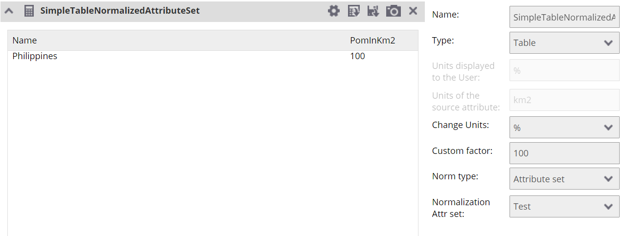
Show the values normalized to the attribute
It is a bit similar to previous choice in the fact that the values from the source attribute are divided by the result attribute. The main difference is that here you are choosing the exact attribute to be used in division. The value is then afterwards multiplied by 100 and shown in percentage, unless specified otherwise.
Outside of the process explained in the documentation of the BackOffice it is also possible to integrate some simple data sources into the visualisation and analysis platform.
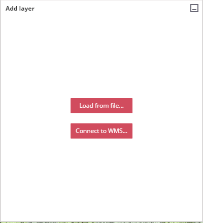
The FrontOffice contains the possibility to show the Custom WMS source alongside the data which are already part of the visualisation and analysis tool.
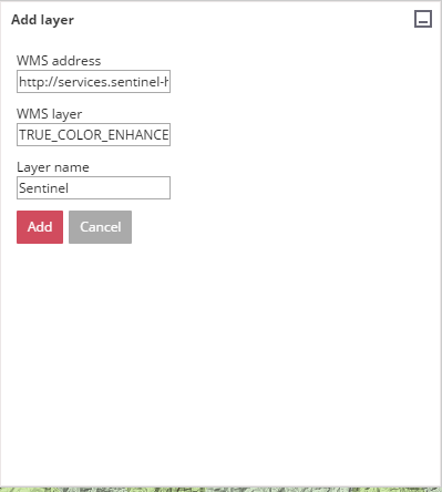
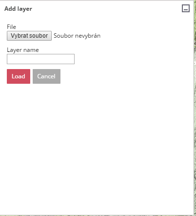
This option for adding the layer will add the layer to current scope to be visualised using default style. It also prepares zonal analysis for the attributes associated to the layer and create averages and sums of the values in the attributes of the layer.
As an expert user it is possible to specify new visualization, which will be available to other users. It is also possible to specify other analysis, which will show the combination of the data received via TEP Urban processing and portal with other types of data already in PUMA. It also supports adding the data via other means than just TEP Urban processing centers.
Further videos documenting how to do this, are available at https://urban-tep.eo.esa.int/puma/backoffice
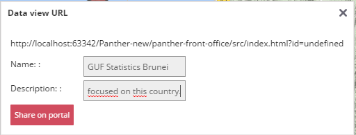
It is possible to integrate results prepared in the Visualisation and analysis tool to the portal for others to query them. It allows the users to publish results in a simple way to the portal via the visualisation and analysis tool.
In order to get to the option click on the share sign on the right. It provides you with the link you can share directly and with the possibility to share into the portal.
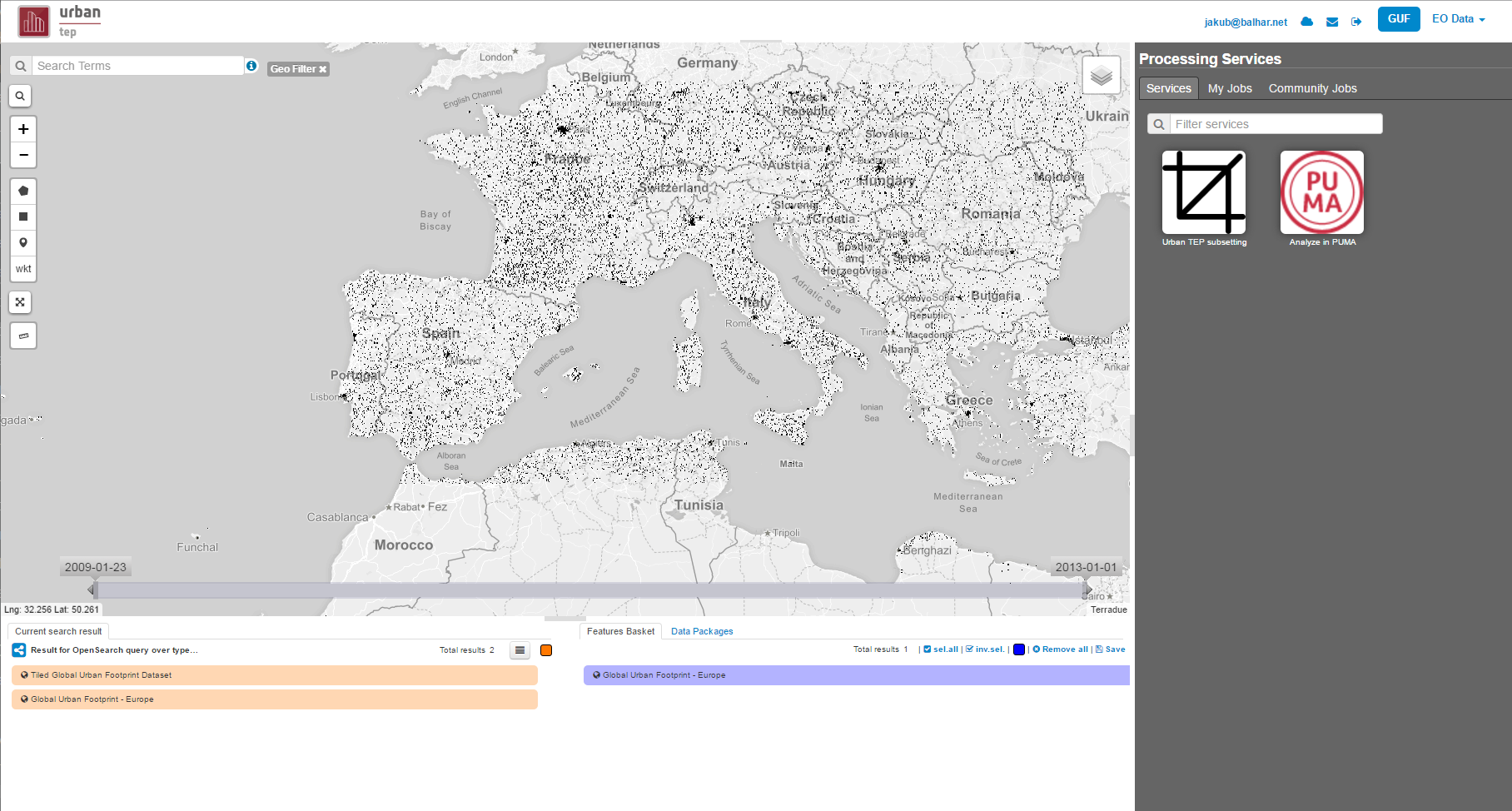
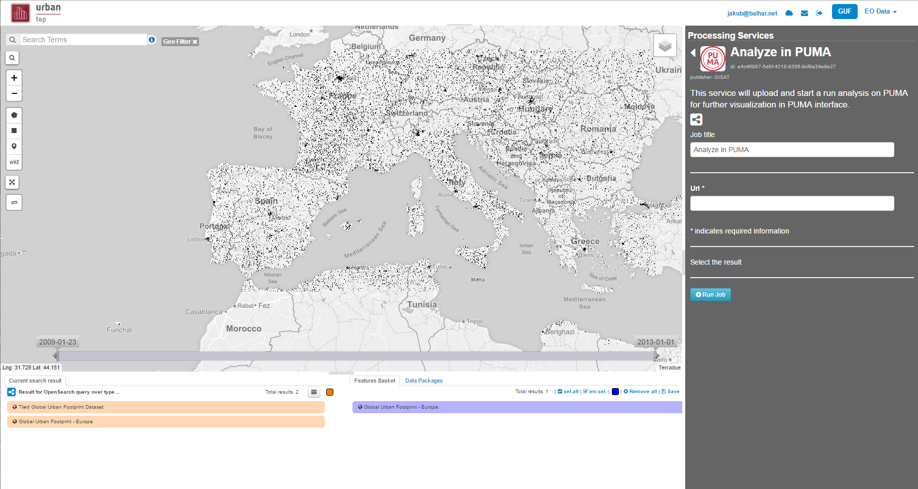
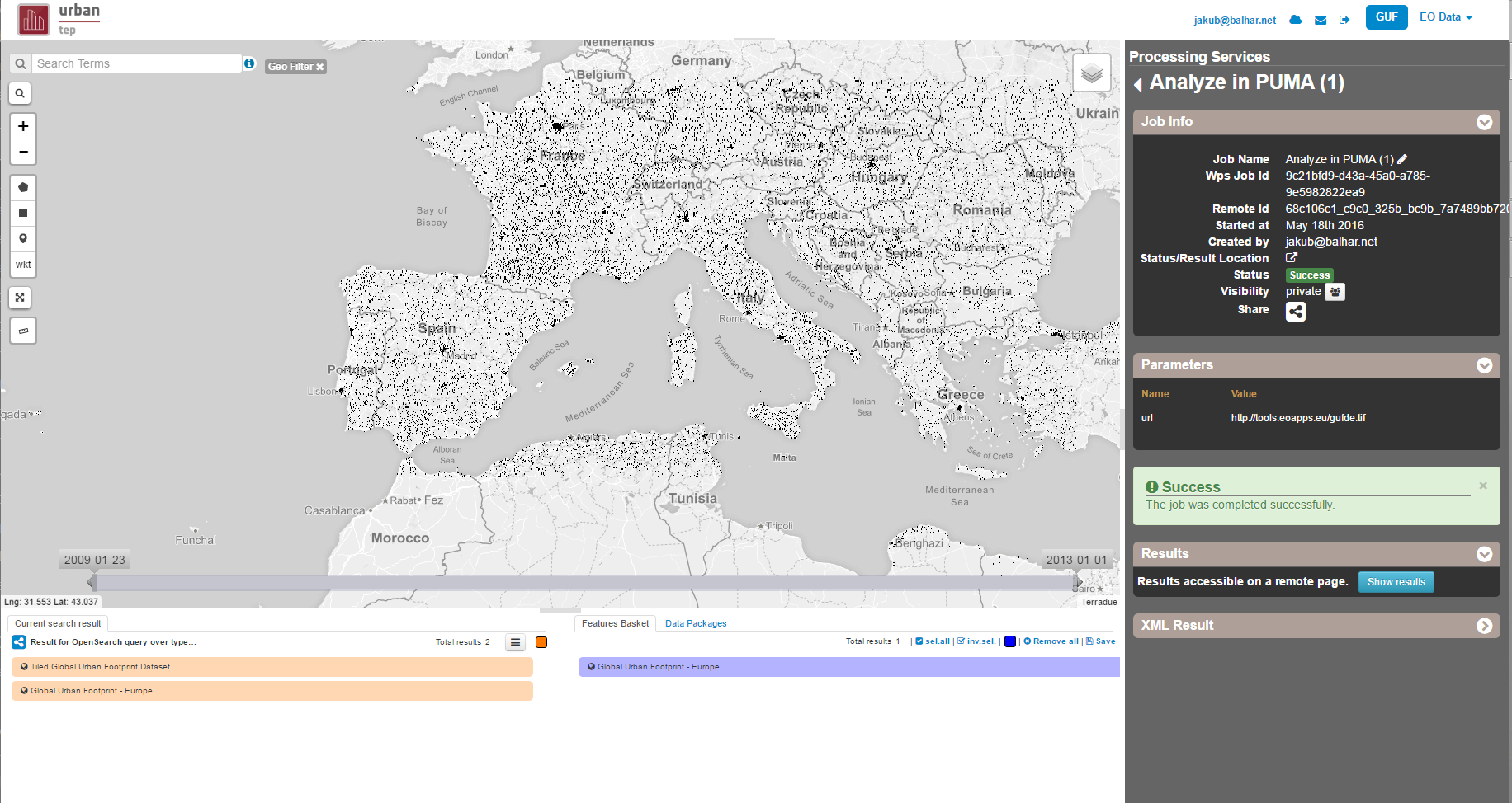
It is possible to import the data into the PUMA using the UrbanTEP portal. It is also then possible to see the data, which were jsut uploaded in the PUMA.
Steps necessary to use Guf subsetting with integration of PUMA.
| show: |
|---|